

Abstract: Since Samuelson’s (1966) reswitching example in the 1960s, it became clear that the Average Production Period (APP) is not necessarily a decreasing function of the interest rate. Recently, Fillieule (2007) and Hülsmann (2010) have shown that Samuelson’s example is not a mere curiosity. They showed that in a reasonable production structure model, the length of production increases with the interest rate instead of decreasing. However, their model did not present “reswitching” behavior. In this paper a generic model of the structure of production, in which both Fillieule’s and Hülsmann’s models are specific cases, is presented. It shows that the APP has a nonmonotonic dependence on the interest rate, which resembles a “reswitching” behavior: it increases for low-interest rates up to a maximum value, and then decreases back to almost the initial value. The decrease occurs within a relatively narrow range of interest rates, which may explain why it was missed in the literature.
business cycle — interest rate — structure of production — austrian economics — reswitching
JEL Classification: B53, E43, L11, L16, D24, B25, L23
Er’el Granot (erel@ariel.ac.il) is a professor at the Department of Electrical and Electronics Engineering, Ariel University, Israel.
INTRODUCTION
Recently, there has been a revival in the interest in the reswitching debate. The debate is part of the Cambridge capital debate, which took place during the 1960s and 1970s (Harcourt 1972, 1976; Cohen and Harcourt 2003). While the capital debate did not end with a clear conclusion, Samuelson (1966) used a nice pedagogical example to illustrate the problem, in what was considered to be one of the main pillars of economics. One of the conclusions of Böhm-Bawerk’s intratemporal studies was that the players’ time preference determines the pure rate of interest (PRI), and therefore when the PRI decreases the entrepreneur seeks more productive roundabout production processes (Böhm-Bawerk 1959). Consequently, it seems that the natural conclusion is that when the PRI decreases, the structure of production lengthens.
This conclusion affected not only the neo-classical school but significantly influenced the Austrian school of thought. Hayek (1933, 1935) developed Jevons’s structure of production and Böhm-Bawerk’s analysis in his business cycle studies. Rothbard (2008) developed Hayek’s treatment by integrating the interest rate in the structure of production. The general structure appears in more modern writings.1
The reswitching debate did not have a considerable impact on the Austrian school, probably because it was not regarded initially as more than a mere curiosity. Moreover, it is true (see Murphy [2003]) that the validity of reswitching does not fundamentally contradict Böhm-Bawerk’s claim that the entrepreneurs’ time-preferences is directly related to their willingness to lengthen or to shorten the production process. In fact, the reswitching effect does not contradict any fundamental praxeological law. However, does it affect the structure of production?
Fillieule (2007) constructed a simple model for the structure of production. In his model the structure of production consists of infinite stages of production, i.e., the structure of production begins at the dawn of humanity. Moreover, it was taken that in every stage the ratio between the amount of money invested in original factors of production (labor and land) and the amount of money invested in capital goods is a given constant ratio.
Under these fundamental propositions, the structure of production has an exponential shape. That is, the structure of production decays exponentially the higher one goes in the production’s stages, since the ratio between the amounts of investment in adjacent stages is fixed. An example of such a production structure is illustrated in Fig. 1.
Figure 1.

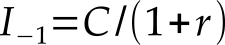
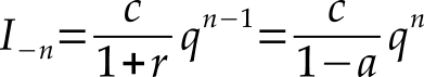
Due to the fixed ratio between adjacent stages of production, the calculation is relatively simple and straightforward. In this case, the Average Production Period (APP) was found to be (Fillieule 2007)
(1) 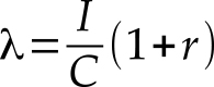
where λ is the APP, I stands for total investment, C is the amount of consumption and r is the interest rate per stage of production.
It should be noted that in the literature the stages are usually numbered by positive numbers, however, to be consistent with the fact that stage 0 is the final stage, I chose to present them as negative numbers. This notation is also consistent with the terminology: “1st stage of production”, “2nd stage of production” etc. 1st cannot correspond to 9, but it may correspond to -9.
Hülsmann (2011) took a similar approach, but with several differences, which have to be stressed. In Hülsmann’s production structure model, there is a finite number of production stages. Furthermore, it is assumed that capitalists pay for original factors of productions (land and labor) only at the beginning of the production process. In the intermediate production stages, capitalists pay only for capital goods plus interest. Furthermore, his research focuses on a low interest rate, in which case the structure of production has a trapezoidal shape (as in Hayek’s model). An example of such a production structure is presented in Fig. 2 (again, one can see that I use negative numbers to represent the stages of production because production takes place in the present).
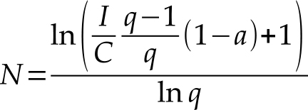
To simplify the discussion, Hülsmann (2011) did not present a formula, and instead, numerical results were presented. However, straightforward derivation reveals that in the low interest regime (the most relevant one, and the one which creates the trapezoidal shape), the dependence of the number of production stages (N) on the interest rate (r) is (see Eq. 6 in Appendix A)
(2) 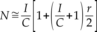
Figure 2.

A more accurate derivation, which is valid for 0 < r < C/I, shows that (these expressions do not appear in the original paper, but are derived in Appendix A as Eqs. A5 and A6).
(3) 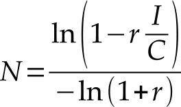
Both the numerator and denominator of Eq. 3 increase with the interest rate, however, since in the numerator r is multiplied by a larger numberIC 1 then the number of stages is an increasing function of the interest rate. Moreover, as r increases and tends toward CI from below, then the number of stages diverges, i.e., N—> ∞.
Therefore, we recognize that in both models the length of production (LOP) increases with the interest rate, which, as was emphasized by Hülsmann, is in clear contrast to the Austrian understanding of the structure of production.
Machaj (2015, 2017) tried to solve the inconsistency between these results and the Austrian literature by emphasizing the importance of the Intertemporal Labor Intensity (ILI) in the production’s structure. According to this terminology, ILI indicates the amount of money being spent on original factors of production in the earlier stages of production relative to the later stages.
High ILI corresponds to the case where most wage payments, i.e. labor investment, are concentrated in the early stages of the production process. Low ILI corresponds to the opposite case, where most wages are paid in the last stages of production. Machaj does not quantify the relation between the ILI and the correlation between the LOP and the interest rate; however, it seems that he relates low ILI with negative correlation and high ILI with a positive one. This tool helps him to explain the positive correlation between the LOP and the interest rate in Hülsmann’s and Fillieule’s model, since, according to him, in both models the ILI is high (see Machaj [2017, 78]).
Clearly, the ILI has an important impact on the structure of production. However, how can it explain the inconsistency between the Austrian literature and the results of Hülsmann and Fillieule? After all, contrary to Machaj’s claim, the ILI is completely different in the two models.
In Hülsmann’s case, the ILI is clearly high (since labor is invested only in the first stage of production). However, in Fillieule’s model, most of the labor investment is concentrated in the last stages of production (after all, there are infinitely many stages, but the labor investment increases exponentially), and therefore the ILI is definitely low, regardless of the interest rate.
Nevertheless, both models present a positive correlation between the LOP and the interest rate (provided the ratio between investment and consumption is fixed).
Therefore, knowing the ILI is insufficient to determine whether the LOP increases or decreases as a function of the interest rate.
Moreover, the ILI is not a well-defined quantity. If ILI is a measure of the average period of labor investment, then it is almost identical to the Böhm-Bawerkian definition of the APP. Then it is clear that the APP is low whenever the ILI is low and vice versa. Therefore, the ILI does not add information to the question about whether the APP will increase or not; the ILI is the solution to this question. But, as we will see below, the situation is even more complicated than that.
Hülsmann emphasized that it is not surprising that in both models the same positive tendency appears, i.e., LOP increases with interest rate, because, according to him, they basically followed the same methodology. However, a close inspection reveals major differences.
Nevertheless, despite the differences between the two models, they are, basically, two specific cases in a more generic one.
CONSTRUCTING THE GENERIC MODEL
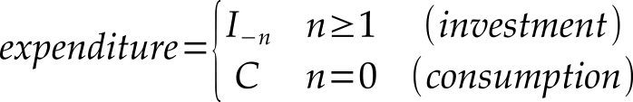
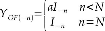
The generic model, is the case where there is a finite number of production stages N (like Hülsmann’s, Hayek’s and Rothbard’s models), but in every production stage the investment consists of capital investment, whose fraction is (1-a), investment in original factors (OF), whose fraction is a (as in Fillieule’s model) and interest fraction r (it should be noted that only when the time period of a single stage is one year does r stand for the annual interest rate). Mathematically, it means that the amount of money capitalists spend in the -nth stage is I-n and the consumption at the final stage (stage zero) is equal to c, i.e.,
(4) 
In the first production stage of high-level goods, the investment is equal to
(5) 
In general, the expenditure on OF of production at the nth stage of production is
(6) 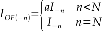
that is, in the intermediate states only a fraction a out of the entire investment is dedicated to OF, while in the first production stage all investment is directed to it.
Therefore, the investment in capital products at the -nth stage of production is
(7) 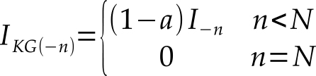
(note that we adopted Fillieule’s notations except for the stages’ numeration).
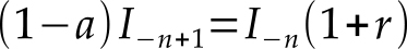
Consequently, the relation between the investments in adjacent stages is (for 2 ≤ n ≤ N)
(8) 
The structure of production of this generic model is presented in Fig. 3.
Figure 3.

This is a generic model: Hülsmann’s model is a specific case, which can be derived by taking the limit of zero expenditure on original factors, i.e. a —> 0, while keeping the number of production stages finite, i.e., N < ∞. Fillieule’s model can be reconstructed by keeping a constant percentage of the expenses on original factors, i.e., a > 0, but taking an infinite number of stages, i.e. N —> ∞. In both models, the interest rate is taken to be non-zero, i.e., r > 0. It should be noted in passing, that the generic model encompasses a third kind of structure, which is reminiscent of Hayek’s (1935) model of the structure of production in that it does not take the interest payments into account, i.e., r = 0. However, it is not the same kind of structure because Hayek’s structure is linear, while the generic model is exponential.
Now, since the LOP in both models (Eqs. 1 and 2) is independent of a we find a problem. Nevertheless, before we explain the problem, we must emphasize again the point that r in our model (as in Fillieule’s and Hülsmann’s) is not the annual interest rate, but rather the interest rate paid in a single production stage. Therefore, if one chooses very short production stages (in the possible range), r can be arbitrarily small regardless of the interest rate (note that the ratio I/C is independent of the length of the stages). In this limit, Fillieule’s result  reveals only a negligible dependence on the interest rate.
In fact, if one follows Fillieule’s derivation with a single difference: omitting the interest rate at the last stage of production, the prefactor (1+r) vanishes, i.e., λ = I/C. Therefore, the dependence on the interest rate (1+r) is a result of the last stage and has nothing to do with the entire (infinitely long) structure of production.
If the number of production stages is finite, then it is clear that in the limit of low interest rate rN << 1 Hülsmann’s model is retrieved, because then Hülsmann’s trapezoid shape appears. However, in the limit of high-interest rate rN >> 1, Fillieule’s model is retrieved, since in these cases the amount of investment in the early stages (n > 1/r ) is minuscule, and therefore for any practical purposes N can go to infinity without affecting the distribution of investment.
Consequently, the parameter which determines in which domains we are is the product Nr. If Nr >> 1 then the model enters Fillieule regime (the production structure is approximately exponential), while when Nr << 1 the model enters Hülsmann’s domain (the production structure is approximately trapezoidal). Clearly, however, our model is richer than the two independent regimes.
Now, we can turn to and explain the problem:
When the interest rate is low, then the APP can be approximated by Eq. 2, i.e. 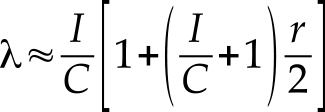 , however, since I/C > 1 then
 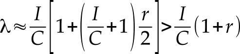 . However, , as was explained above, should be valid for higher interest rates, when the number of stages diverges. Therefore, for any given interest rate, Hülsmann’s model APP is higher than Fillieule’s, which means that eventually, the APP must decrease. Below we will present this behavior in detail.
The inevitable conclusion is that the two formulae do not present the same reality, and not even the same tendency. In fact, these results show that for low interest rates, the LOP increases with the interest rate, while for high interest rates the LOP must decrease. The mathematical proof for this will be presented below.
There is no monotonic dependence on the interest rate. Therefore, not only do these models contradict the Austrian and neo-classical literature, but a reswitching >musteventually occur. Reswitching is, then, not an anomaly or a mere curiosity, but it is the norm (provided the ratio between consumption and investment is fixed).
It should be stressed, however, that this “reswitching” is not equivalent to Samuelson’s original one. This is because the reswitching does not occur between two different production methods, but rather a reswitching occurs in the sense that for low interest rates the production structure is short; when the interest rate increases the structure of production lengthens. However, it shrinks again when the interest rate keeps increasing.
One of the reasons that this unexpected conduct was overlooked is that there are inconsistencies in the definitions of the LOP.
In what follows, we will solve this model analytically, and present the reswitching result. However, before we do that, we have to clear up the confusion regarding the definition of the LOP.
Jevons, Hayek, Rothbard, and Hülsmann identified the LOP with the number of production stages. When the number of stages is low, i.e., when N(α+r) << 1, the number of stages is indeed a very good estimation to the LOP. However, when the number of stages increases, the amount of money invested in the early stages of production, i.e., where higher-level goods are produced, is small in comparison to the aggregate investment. Therefore, the contribution of these stages to the LOP is negligible. Clearly, when the number of stages is infinite, i.e., when the production process begins at the dawn of humanity (as in Fillieule’s model), it is clear that the number of stages is an inadequate evaluation of the LOP.
It should be stressed that taking the production stages to infinity is not merely an academic exercise. In fact, as was stressed by Machaj (2017), any modern production process begins with capital goods. It is almost impossible to reconstruct a production process that does not require capital goods in its initial production stage. Therefore, an infinite number of stages does not seem to be the exception, but rather seems to be the norm, and should not be disregarded.
Ironically, it seems that Böhm-Bawerk has realized this problem, and used the average period of production, which is defined as the “average time interval occurring between each expenditure of originary productive forces and the final completion of the ultimate consumption good.” Therefore, instead of using the ambiguous term LOP, we would use the more clearly defined term “average period of production” (APP). This term can easily be implemented in all three models by
(9) 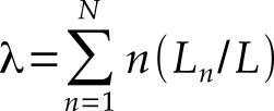
where Ln is the amount of money invested in labor during the nth stage of production, while
(10) 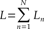
is the aggregate investment in original factors (labor and land).
Hereinafter we will adopt Fillieule’s assumption that in the intermediate stages all the investment on OF consists of labor’s salaries. This is a reasonable assumption because it is very rare that the industries utilize unprocessed OF, i.e. non-capital goods, during intermediate stages of production. Moreover, it is not a restrictive assumption, and the model can easily be generalized.
CALCULATION OF THE APP
From Eqs. 5 and 8, the investment in the nth stage can easily be calculated:
(11) 
for n ≥ 1, where, for simplicity, the following notation was used
(12) 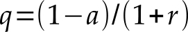 .
.
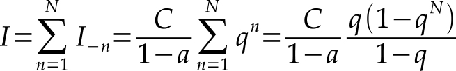
Then, aggregate saving is (see Appendix A)
(14) 
Similarly, the aggregate income of owners of OF is
(15) 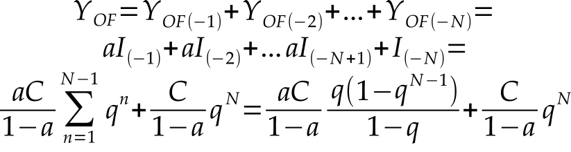
where
(16)  ,
,
are the incomes of owners of OF in the -nth stage, which is a manifestation of the fact that in the Nth production stage all money is invested in OF, while in the intermediate stages only part (a) of the money is invested in them.
Similarly, the aggregate income of owners of capital goods is equal to
(17)  .
.
Using Eq. 9 the APP is (see Appendix A)
(18) 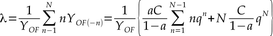
which can be solved as
(19) 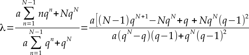
The dependence of the APP on the interest rate is via the auxiliary parameter q.
According to Eq. 19 when the parameters a and N are fixed then λ (the APP) decreases when the interest rate r increases. However, when the interest rate varies, so does the aggregate investment I (according to Eq. 14).
In order to keep the aggregate investment fixed, the number of stages of production N must increase accordingly. Therefore, in order to keep the ratio between consumption and investment fixed, one can substitute the number of stages N from Eq. 14 into Eq. 19, i.e., to substitute
(20) 
in the expression for λ, (note that Eq. 3 is a specific case when a=0). But before we do it, it is useful to adopt the following definition of the critical interest rate
(21)  .
.
Using this terminology, the number of production stages, i.e., Eq. 20, can be written
(22)  .
.
which clearly diverges when r —> rc.
By substituting Eqs. 12, 21, and 22 in Eq. 19 the APP can finally be written as (see Appendix B for elaboration)
(23) 
When a —> 0 then λ —> N, i.e., the APP converges to the number of stages. In fact, as long asr << rc and a << r then λ ≅ N (see Eq. B2 in Appendix B), i.e., in this case, the number of production stages is indeed a good approximation of the APP. This is the interest rate regime, which was investigated by Hülsmann.
However, as the interest rate approaches the critical interest rate, i.e., r ≅ rc, then the number of stages N diverges, while the APP, i.e. λ, does not (see Fig. 4). In fact, the APP finally decreases and converges to (note that all the terms (rc-r) in Eq. 23 vanish)
(24) 
which is exactly Fillieule’s (2007) result for r ≅ rc .
In context of the generic model, which is presented in this paper, we see that Hülsmann and Fillieule investigated different regimes of the interest rate. Hülsmann’s model agrees with the generic model at the low interest rate regime, while Fillieule’s model agrees with the generic model only around r ≅ rc, where the number of stages diverges.
As can be seen from Fig. 4, there is an interest rate level r*, below which the APP increases, and above which the APP decreases. This is the point where APP receives its maximum value λmax = λ(r*) (see Fig. 4).
Figure 4.

In Fig. 5, the APP as a function of a and r is presented in a contour plot. As can be seen, for any given 0 < a < C/I there is an interest rate, which is lower than the critical one, in which the APP receives its maximum value, and above which it decreases to almost the initial value.
Figure 5.

This maximum effect is especially noticeable when the fraction of OF’s investment is very low, i.e., a << 1 (For details, see Appendix C).
This “reswitching” phenomenon occurs due to the following reasons. In the low interest rate regime, any increase in the interest rate forces the APP to expand in order to compensate for the reduction in the high-level stages of investment. However, this process cannot last for long, since when the interest rate increases beyond a certain level (r*), the reduction in the low stages’ investment reduces the APP beyond the increase caused by the additional stages. Thus, in this regime, the APP decreases. Beyond the critical interest rate (rc) the reduction in the low stages’ investment cannot be compensated by the negligible investment in the high stages of production.
It should be emphasized that when r < rc the interest rate can increase while both I/C and a are fixed, because the number of stages can increase. However, beyond rc, since the number of stages is already infinite, it is impossible to raise the interest rate without affecting either a or I/C. In this regime, if the ratio I/C is fixed, then λ = (I/C)(1+r) (Eq. 1), in which case the APP mildly increases with the interest rate (see the dashed curve in Fig. 6). However, if a is fixed, then APP obeys the equation λ = (1+r)/(r+a) (see Fillieule [2007]), in which case the APP decreases with the interest rate (see the solid curve in Fig. 6).
Figure 6.

A further important and original result is, that the APP does not have a simple monotonic decreasing dependence on the ratio between consumption and investment (as wrongly predicted in the literature, see, for example, Chapter 8 in Murphy [2006]). If the fraction a and the interest rate r are fixed, the APP initially increases with the ratio (C/I), and only after receiving its maximum value, it begins to decrease (as N does); see Fig. 7.
Figure 7.

In countries like the United States where C/I ≈ 0.5 (see Skousen [1991, 45]) the difference between rc ≡ C/I a, and r* (the interest rate with the longest APP) is very small (see Fig. 8 where r* was calculated numerically).
Figure 8.

This fact can explain why this “reswitching” was missed in the literature, and how it became common knowledge that the APP must decrease when the interest rate increases.
SUMMARY AND CONCLUSION
A generic model of the structure of production was presented and studied. Hülsmann’s and Fillieule’s models are two limiting cases of the generic model. The low interest regime of the generic model can be approximated by Hülsmann’s model, while the high interest regime of the generic model can be approximated by Fillieule’s model.
Thus, the generic model leads to a result that is different both from the older Austrian literature and from the recent one.
Therefore, this model predicts that when the interest rate increases, the APP does not decrease as the neo-classical models (and the old Austrian literature) predict. Moreover, the APP does not increase as the new Austrian models predict.
In fact, the main prediction is that when the ratio between consumption and investment is fixed, the APP increases for low interest rates, but beyond a certain value, it decreases.
This conduct resembles a “reswitching” behavior when the APP is low for both low and high interest rates, but it grows for intermediate interest rate levels.
However, this conduct can occur only if the ratio between consumption and investment (C/I) and a are both fixed, which is possible to maintain only within a narrow range of interest rate values. Whenever the interest rate exceeds this range, at least one of these parameters, either (C/I) or a, must vary as well. If the former (C/I) is fixed, then the recent Austrian prediction holds, but when the latter (a) is fixed, then the older Austrian prediction is valid.
- 1See, e.g., Skousen (1990), de Soto (2006).
