7. Production: General Pricing of the Factors
7. Production: General Pricing of the Factors1. Imputation of the Discounted Marginal Value Product
1. Imputation of the Discounted Marginal Value ProductUP TO THIS POINT, WE have been investigating the rate of interest as it would be determined in the evenly rotating economy, i.e., as it always tends to be determined in the real world. Now we shall investigate the pricing of the various factors of production in the same terms, i.e., as they tend to be in the real world, and as they would be in the evenly rotating economy.
Whenever we have touched on the pricing of productive factors we have signified the prices of their unit services, i.e., their rents. In order to set aside consideration of the pricing of the factors as “wholes,” as embodiments of a series of future unit services, we have been assuming that no businessmen purchase factors (whether land, labor, or capital goods) outright, but only unit services of these factors. This assumption will be continued for the time being. Later on, we shall drop this restrictive assumption and consider the pricing of “whole factors.”
In chapter 5 we saw that when all factors are specific there is no principle of pricing that we can offer. Practically, the only thing that economic analysis can say about the pricing of the productive factors in such a case is that voluntary bargaining among the factor-owners will settle the issue. As long as the factors are all purely specific, economic analysis can say little more about the determinants of their pricing. What conditions must apply, then, to enable us to be more definite about the pricing of factors?
The currently fashionable account of this subject hinges on the fixity or variability in the proportions of the combined factors used per unit of product. If the factors can be combined only in certain fixed proportions to produce a given quantity of product, it is alleged, then there can be no determinate price; if the proportions of the factors can be varied to produce a given result, then the pricing of each factor can be isolated and determined. Let us examine this contention. Suppose that a product worth 20 gold ounces is produced by three factors, each one purely specific to this production. Suppose that the proportions are variable, so that a product worth 20 gold ounces can be produced either by four units of factor A, five units of factor B, and three units of factor C, or by six units of A, four units of B, and two units of C. How will this help the economist to say anything more about the pricing of these factors than that it will be determined by bargaining? The prices will still be determined by bargaining, and it is obvious that the variability in the proportions of the factors does not aid us in any determination of the specific value or share of each particular product. Since each factor is purely specific, there is no way we can analytically ascertain how a price for a factor is obtained.
The fallacious emphasis on variability of proportion as the basis for factor pricing in the current literature is a result of the prevailing method of analysis. A typical single firm is considered, with its selling prices and prices of factors given. Then, the proportions of the factors are assumed to be variable. It can be shown, accordingly, that if the price of factor A increases compared to B, the firm will use less of A and more of B in producing its product. From this, demand curves for each factor are deduced, and the pricing of each factor established.
The fallacies of this approach are numerous. The chief error is that of basing a causal explanation of factor pricing on the assumption of given factor prices. On the contrary, we cannot explain factor prices while assuming them as given from the very beginning of the analysis.1 It is then assumed that the price of a factor changes. But how can such a change take place? In the market there are no uncaused changes.
It is true that this is the way the market looks to a typical firm. But concentration on a single firm and the reaction of its owner is not the appropriate route to the theory of production; on the contrary, it is likely to be misleading, as in this case. In the current literature, this preoccupation with the single firm rather than with the interrelatedness of firms in the economy has led to the erection of a vastly complicated and largely valueless edifice of production theory.
The entire discussion of variable and fixed proportions is really technological rather than economic, and this fact should have alerted those writers who rely on variability as the key to their explanation of pricing.2 The one technological conclusion that we know purely from praxeology is the law of returns, derived at the beginning of chapter 1. According to the law of returns, there is an optimum of proportions of factors, given other factors, in the production of any given product. This optimum may be the only proportion at which the good can be produced, or it may be one of many proportions. The former is the case of fixed proportions, the latter of variable proportions. Both cases are subsumed under the more general law of returns, and we shall see that our analysis of factor pricing is based only on this praxeological law and not on more restrictive technological assumptions.
The key question, in fact, is not variability, but specificity of factors.3 For determinate factor pricing to take place, there must be nonspecific factors, factors that are useful in several production processes. It is the prices of these nonspecific factors that are determinate. If, in any particular case, only one factor is specific, then its price is also determined: it is the residual difference between the sum of the prices of the nonspecific factors and the price of the common product. When there is more than one specific factor in each process, however, only the cumulative residual price is determined, and the price of each specific factor singly can be determined solely by bargaining.
To arrive at the principles of pricing, let us first leap to the conclusion and then trace the process of arriving at this conclusion. Every capitalist will attempt to employ a factor (or rather, the service of a factor) at the price that will be at least less than its discounted marginal value product. The marginal value product is the monetary revenue that may be attributed, or “imputed,” to one service unit of the factor. It is the “marginal” value product, because the supply of the factor is in discrete units. This MVP (marginal value product) is discounted by the social rate of time preference, i.e., by the going rate of interest. Suppose, for example, that a unit of a factor (say a day’s worth of a certain acre of land or a day’s worth of the effort of a certain laborer) will, imputably, produce for the firm a product one year from now that will be sold for 20 gold ounces. The MVP of this factor is 20 ounces. But this is a future good. The present value of the future good, and it is this present value that is now being purchased, will be equal to the MVP discounted by the going rate of interest. If the rate of interest is 5 percent, then the discounted MVP will be equal to 19 ounces. To the employer—the capitalist—then, the maximum amount that the factor unit is now worth is 19 ounces. The capitalist will be willing to buy this factor at any price up to 19 ounces.
Now suppose that the capitalist owner or owners of one firm pay for this factor 15 ounces per unit. As we shall see in greater detail later on, this means that the capitalist earns a pure profit of four ounces per unit, since he reaps 19 ounces from the final sale. (He obtains 20 ounces on final sale, but one ounce is the result of his time preference and waiting and is not pure profit; 19 ounces is the present value of his final sale.) But, seeing this happen, other entrepreneurs will leap into the breach to reap these profits. These capitalists will have to bid the factor away from the first capitalist and thus pay more than 15 ounces, say 17 ounces. This process continues until the factor earns its full DMVP (discounted marginal value product), and no pure profits remain. The result is that in the ERE every isolable factor will earn its DMVP, and this will be its price. As a result, each factor will earn its DMVP, and the capitalist will earn the going rate of interest for purchasing future goods with his savings. In the ERE, as we have seen, all capitalists will earn the same going rate of interest, and no pure profit will then be reaped. The sale price of a good will be necessarily equal to the sum of the DMVPs of its factors plus the rate of interest return on the investment.
It is clear that if the marginal value of a specific unit of factor service can be isolated and determined, then the forces of competition on the market will result in making its price equal to its DMVP in the ERE. Any price higher than the discounted marginal value product of a factor service will not long be paid by a capitalist; any price lower will be raised by the competitive actions of entrepreneurs bidding away these factors through offers of higher prices. These actions will lead, in the former case to the disappearance of losses, in the latter, to the disappearance of pure profit, at which time the ERE is reached.
When a factor is isolable, i.e., if its service can be separated out in appraised value from other factors, then its price will always tend to be set equal to its DMVP. The factor is clearly not isolable, if, as mentioned in note 3 above, it must always be combined with some other particular factor in fixed proportions. If this happens, then a price can be given only to the cumulative product of the factors, and the individual price can be determined only through bargaining. Also, as we have stated, if the factors are all purely specific to the product, then, regardless of any variability in the proportions of their combination, the factors will not be isolable.
It is, then, the nonspecific factors that are directly isolable; a specific factor is isolable if it is the only specific factor in the combination, in which case its price is the difference between the price of the product and the sum of the prices of the nonspecific factors. But by what process does the market isolate and determine the share (the MVP of a certain unit of a factor) of income yielded from production?
Let us refer back to the basic law of utility. What will be the marginal value of a unit of any good? It will be equal to the individual’s valuation of the end that must remain unattained should this unit be removed. If a man possesses 20 units of a good, and the uses served by the good are ranked one to 20 on his value scale (one being the ordinal highest), then his loss of a unit—regardless of which end the unit is supplying at present—will mean a loss of the use ranked 20th in his scale. Therefore, the marginal utility of a unit of the good is ranked at 20 on the person’s value scale. Any further unit to be acquired will satisfy the next highest of the ends not yet being served, i.e., at 21—a rank which will necessarily be lower than the ends already being served. The greater the supply of a good, then, the lower the value of its marginal utility.
A similar analysis is applicable to a producers’ good as well. A unit of a producers’ good will be valued in terms of the revenue that will be lost should one unit of the good be lost. This can be determined by an entrepreneur’s knowledge of his “production function,” i.e., the various ways in which factors can technologically be combined to yield certain products, and his estimate of the demand curve of the buyers of his product, i.e., the prices that they would be willing to pay for his product. Suppose, now, that a firm is combining factors in the following way:
4X + 10Y + 2Z → 100 gold oz.
Four units of X plus 10 units of Y plus two units of Z produce a product that can be sold for 100 gold ounces. Now suppose that the entrepreneur estimates that the following would happen if one unit of X were eliminated:
3X + 10Y + 2Z → 80 gold oz.
The loss of one unit of X, other factors remaining constant, has resulted in the loss of 20 gold ounces of gross revenue. This, then, is the marginal value product of the unit at this position and with this use.4
This process is reversible as well. Thus, suppose the firm is at present producing in the latter proportions and reaping 80 gold ounces. If it adds a fourth unit of X to its combination, keeping other quantities constant, it earns 20 more gold ounces. So that here as well, the MVP of this unit is 20 gold ounces.
This example has implicitly assumed a case of variable proportions. What if the proportions are necessarily fixed? In that case, the loss of a unit of X would require that proportionate quantities of Y, Z, etc., be disposed of. The combination of factors built on 3X would then be as follows:
3X + 7.5Y + 1.5Z → 75 gold oz. (assuming no price change in the final product)
With fixed proportions, then, the marginal value product of the varying factor would be greater, in this case 25 gold ounces.5
Let us for the moment ignore the variations in MVP within each production process and consider only variations in MVP among different processes. This is basic since, after all, it is necessary to have a factor usable in more than one production process before its MVP can be isolated. Inevitably, then, the MVP will differ from process to process, since the various production combinations of factors and prices of products will differ. For every factor, then, there is available a sheaf of possible investments in different production processes, each differing in MVP. The MVPs (or, strictly, the discounted MVPs), can be arrayed in descending order. For example, for factor X:
25 oz.
24 oz.
22 oz.
21 oz.
20 oz.
19 oz.
18 oz.
etc.
Suppose that we begin in the economy with a zero supply of the factor, and then add one unit. Where will this one unit be employed? It is obvious that it will be employed in the use with the highest DMVP. The reason is that capitalists in the various production processes will compete with one another for the use of the factor. But the use in which the DMVP is 25 can bid away the unit of the factor from the other competitors, and it can do this finally only by paying 25 gold ounces for the unit. When the second unit of supply arrives in society, it goes to the second highest use, and it receives a price of 24 ounces, and a similar process occurs as new units of supply are added. As new supply is added, the marginal value product of a unit declines. Conversely, if the supply of a factor decreases (i.e., the total supply in the economy), the marginal value product of a unit increases. The same laws apply, of course, to the DMVP, since this is just the MVP discounted by a common factor, the market’s pure rate of interest. As supply increases, then, more and more of the sheaf of available employments for the factor are used, and lower and lower MVPs are tapped.
Diagrammatically, we may see this situation as in Figure 56.
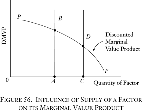
The line PP is the curve of the marginal value product (or discounted MVP) of a factor. It is always declining as it moves to the right, because new units of supply always enter those uses that are most productive of revenue. On the horizontal axis is the quantity of supply of the factor. When the supply is 0A, then the MVP is AB. When the supply is larger at 0C, then the MVP is lower at CD.
Let us say that there are 30 units of factor X available in the economy, and that the MVP corresponding to such a supply is 10 ounces. The price of the 30th unit, then, will tend to be 10 ounces and will be 10 ounces in the ERE. This follows from the tendency of the price of a factor to be equal to its MVP. But now we must recall that there takes place the inexorable tendency in the market for the price of all units of any good to be uniform throughout its market. This must apply to a productive factor just as to any other good. Indeed, this result follows from the very basic law of utility that we have been considering. For, since factor units by definition are interchangeable, the value of one unit will be equal to the value of every other unit at any one time. The value of every unit of a good will be equal to the value of the lowest-ranking use now served by a unit. In the present case, every unit of the factor will be priced at 10 gold ounces.
Suppose, for example, that the owner of the factor unit serving the top-ranking use in our array should demand that he receive 24 ounces, instead of 10 ounces, as his price. In that case, the capitalist in that line of production can refuse to hire this factor and instead bid away the unit employed in the lowest-ranking use, say by paying for the latter 10.5 ounces. The only alternative left to the owner of the factor who had demanded 24 ounces is to replace the other factor in the lowest-ranking spot, at 10 ounces. Effectively, all factors will shift until the prices that they can attain will be uniform throughout the market for their services.
The price of X, then, is determined at 10 ounces. It is determined by the MVP (or rather the DMVP) of the supply, which decreases as the supply increases, and vice versa. Let us assume that Y is also a nonspecific factor and that Z is a factor specific to the particular process considered above. Let us further assume that, by a similar process, the DMVP, and therefore the price, of Y is determined at two ounces.
At this point, we must reintroduce the concept of production within each line. We have been discussing MVPs of factors shifted from one use to another. In our example, a unit of X may have an MVP (or DMVP) of 20 ounces in a particular use; yet its price, as determined by the MVP of the lowest-ranking use for which it is employed, is 10 ounces. This means that, in this use, the capitalist is hiring a factor for 10 ounces which earns for him 20 ounces. Spurred on by this profit, he will hire more units of the factor until the MVP in this use will equal the MVP in the lowest-ranking use, i.e., the factor price, 10 ounces. The same process will occur in regard to each of the other uses. The tendency will always be, then (and this will always obtain in the ERE), for the DMVP of any factor to be equal in each line of production. We will see shortly why increased purchase of a factor even within each line will lower the MVP in that line.
Suppose, then, that the prices of X and Y are 10 and two ounces respectively and that all the capitalists have so arranged their production as to equate the DMVP of each factor in each line with this price. Suppose, further, that the equilibrium point in this particular use is the combination:
3X + 10Y + 2Z → 80 oz.
Substituting the given prices of X and Y:
3 + 20 + 2Z → 80 oz.
2Z → 80 oz.
Z → 80 oz.
Therefore, Z = 15 oz.
The price of the specific factor Z, residual to the other factors, is thereby determined at 15 ounces.
It is obvious that the impact of a change in consumer demand on a specific factor will be far greater, in either direction, than it will be on the price of employment of a nonspecific factor.
It is now clear why the temptation in factor-price analysis is for the firm to consider that factor prices are given externally to itself and that it simply varies its production in accordance with these prices. However, from an analytic standpoint, it should be evident that the array of MVPs as a whole is the determining factor, and the lowest-ranking process in terms of MVP will, through the medium of factor prices, transmit its message, so to speak, to the various firms, each of which will use the factor to such an extent that its DMVP will be brought into alignment with its price. But the ultimate determining factor is the DMVP schedule, not the factor price. To make the distinction, we may term the full array of all MVPs for a factor, the general DMVP schedule of a factor, while the special array of DMVPs within any particular production process or stage, we may term the particular DMVP schedule of the factor. It is the general DMVP schedule that determines the price of the supply of the factor, and then the particular DMVP schedules within each production process are brought into alignment so that the DMVPs of the factor equal its price. Figure 56 above was a general schedule. The particular MVPs are subarrays within the widest array of all the possible alternatives—the general MVP schedule.
In short, the prices of productive factors are determined as follows: Where a factor is isolable, its price will tend toward its discounted marginal value product and will equal its DMVP in the ERE. A factor will be isolable where it is nonspecific, i.e., is useful in more than one productive process, or where it is the only specific factor in a process. The nonspecific factor’s price will be set equal to its DMVP as determined by its general DMVP schedule: the full possible array of DMVPs, given various units of supply of the factor in the economy. Since the most value-productive uses will be chosen first, and the least abandoned first, the curve of general MVP declines as the supply increases. The various particular MVPs in the various processes will be arranged so as to equal the factor price set by the general DMVP schedule. The specific factor’s imputed DMVP is the residual difference between the price of the product and the sum of the prices of the nonspecific factors.
The marginal utility of a unit of a good is determined by a man’s diminishing marginal utility schedule evaluating a certain supply or stock of that good. Similarly, the market’s establishment of the price of a consumers’ good is determined by the aggregate consumer demand schedules—diminishing—and their intersection with the given supply or stock of a good. We are now engaged in pursuing the problem still further and in finding the answer to two general questions: What determines the prices of factors of production on the market, and what determines the quantity of goods that will be produced? We have seen in this section that the price of a factor is determined by its diminishing general (discounted) marginal value productivity curve intersecting with the given supply (stock) of the factor in the economy.
- 1The mathematical bent toward replacing the concepts of cause and effect by mutual determination has contributed to the willingness to engage in circular reasoning. See Rothbard, “Toward a Reconstruction of Utility and Welfare Economics,” p. 236; and Kauder, “Intellectual and Political Roots of the Older Austrian School.”
- 2Clearly, the longer the period of time, the more variable will factor proportions tend to be. Technologically, varying amounts of time are needed to rearrange the various factors.
- 3This justifies the conclusion of Mises, Human Action, p. 336, as compared, for example, with the analysis in George J. Stigler’s Production and Distribution Theories. Mises adds the important proviso that if the factors have the same fixed proportions in all the processes for which they are nonspecific, then here too only bargaining can determine their prices.
- 4Strictly, we should be dealing with discounted MVPs here, but treating just MVPs at this stage merely simplifies matters.
- 5We are here postulating that equal quantities of factors produce equal quantities of results. The famous question whether this condition actually holds (sometimes phrased in pretentious mathematical language as whether the “production function is linear and homogeneous”) is easily resolved if we realize that the proposition: equal causes produce equal results, is the major technological axiom in nature. Any cases that appear to confute this rule only do so in appearance; in reality, supposed exceptions always involve some “indivisibility” where one factor, in effect, cannot change proportionately with other factors.
2. Determination of the Discounted Marginal Value Product
2. Determination of the Discounted Marginal Value ProductA. Discounting
A. DiscountingIf the DMVP schedules determine the prices of nonspecific factor services, what determines the shape and position of the DMVP schedules? In the first place, by definition it is clear that the DMVP schedule is the MVP schedule for that factor discounted. There is no mystery about the discounting; as we have stated, the MVP of the factor is discounted in accordance with the going pure rate of interest on the market. The relation of the MVP schedule and the DMVP schedule may be diagrammed as in Figure 57.
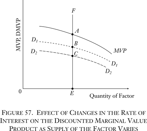
The supply of the factor is the EF line at the given quantity 0E. The solid line is the MVP schedule at various supplies. The MVP of the supply 0E is EA. Now the broken line D1D1 is the discounted marginal value product schedule at a certain rate of interest. Since it is discounted, it is uniformly lower than the MVP curve. In absolute terms, it is relatively lower at the left of the diagram, because an equal percentage drop implies a greater absolute drop where the amount is greater. The DMVP for supply 0E equals EB. EB will be the price of the factor in the evenly rotating economy.
Now suppose that the rate of interest in the economy rises, as a result, of course, of rises in time-preference schedules. This means that the rate of discount for every hypothetical MVP will be greater, and the absolute levels lower. The new DMVP schedule is depicted as the dotted line D2D2. The new price for the same supply of the factor is EC, a lower price than before.
One of the determinants of the DMVP schedule, then, is the rate of discount, and we have seen above that the rate of discount is determined by individual time preferences. The higher the rate of discount, the lower will tend to be the DMVP and, therefore, the lower the price of the factor; the lower the interest rate, the higher the DMVP and the price of the factor.
B. The Marginal Physical Product
B. The Marginal Physical ProductWhat, then, determines the position and shape of the MVP schedule? What is the marginal value product? It is the amount of revenue intake attributable to a unit of a factor. And this revenue depends on two elements: (1) the physical product produced and (2) the price of that product. If one hour of factor X is estimated by the market to produce a value of 20 gold ounces, this might be because one hour produces 20 units of the physical product, which are sold at a price of one gold ounce per unit. Or the same MVP might result from the production of 10 units of the product, sold at two gold ounces per unit, etc. In short, the marginal value product of a factor service unit is equal to its marginal physical product times the price of that product.6
Let us, then, investigate the determinants of the marginal physical product (MPP). In the first place, there can be no general schedule for the MPP as there is for the MVP, for the simple reason that physical units of various goods are not comparable. How can a dozen eggs, a pound of butter, and a house be compared in physical terms? Yet the same factor might be useful in the production of any of these goods. There can be an MPP schedule, therefore, only in particular terms, i.e., in terms of each particular production process in which the factor can be engaged. For each production process there will be for the factor a marginal physical production schedule of a certain shape. The MPP for a supply in that process is the amount of the physical product imputable to one unit of that factor, i.e., the amount of the product that will be lost if one unit of the factor is removed. If the supply of the factor in the process is increased by one unit, other factors remaining the same, then the MPP of the supply becomes the additional physical product that can be gained from the addition of the unit. The supply of the factor that is relevant for the MPP schedules is not the total supply in the society, but the supply in each process, since the MPP schedules are established for each process separately.
- 6This is not strictly true, but the technical error in the statement does not affect the causal analysis in the text. In fact, this argument is strengthened, for MVP actually equals MPP × “marginal revenue,” and marginal revenue is always less than, or equal to, price. See Appendix A below, “Marginal Physical and Marginal Value Product.”
(1) The Law of Returns
(1) The Law of ReturnsIn order to investigate the MPP schedule further, let us recall the law of returns, set forth in chapter 1. According to the law of returns, an eternal truth of human action, if the quantity of one factor varies, and the quantities of other factors remain constant, there is a point at which the physical product per factor is at a maximum. Physical product per factor may be termed the average physical product (APP). The law further states that with either a lesser or a greater supply of the factor the APP must be lower. We may diagram a typical APP curve as in Figure 58.

(2) Marginal Physical Product and Average Physical Product
(2) Marginal Physical Product and Average Physical ProductWhat is the relationship between the APP and MPP? The MPP is the amount of physical product that will be produced with the addition of one unit of a factor, other factors being given. The APP is the ratio of the total product to the total quantity of the variable factor, other factors being given. To illustrate the meanings of APP and MPP, let us consider a hypothetical case in which all units of other factors are constant, and the number of units of one factor is variable. In Table 13 the first column lists the number of units of the variable factor, and the second column the total physical product produced when these varying units are combined with fixed units of the other factors. The third column is the APP = total product divided by the number of units of the factor, i.e., the average physical productivity of a unit of the factor. The fourth column is the MPP = the difference in total product yielded by adding one more unit of the variable factor, i.e., the total product of the current row minus the total product of the preceding row:
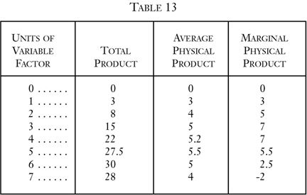
In the first place, it is quite clear that no factor will ever be employed in the region where the MPP is negative. In our example, this occurs where seven units of the factor are being employed. Six units of the factor, combined with given other factors, produced 30 units of the product. An addition of another unit results in a loss of two units of the product. The MPP of the factor when seven units are employed is -2. Obviously, no factor will ever be employed in this region, and this holds true whether the factor-owner is also owner of the product, or a capitalist hires the factor to work on the product. It would be senseless and contrary to the principles of human action to expend either effort or money on added factors only to have the quantity of the total product decline.
In the tabulation, we follow the law of returns, in that the APP, beginning, of course, at zero with zero units of the factor, rises to a peak and then falls. We also observe the following from our chart: (1) when the APP is rising (with the exception of the very first step where T P, APP, and MPP are all equal) MPP is higher than APP; (2) when the APP is falling, MPP is lower than APP; (3) at the point of maximum APP, MPP is equal to APP. We shall now prove, algebraically, that these three laws always hold.7
Let F be any number of units of a variable factor, other factors being given, and P be the units of the total product yielded by the combination. Then P/F is the Average Physical Product. When we add ΔF more units of the factor, total product increases by ΔP. Marginal Physical Product corresponding to the increase in the factor is ΔP/ΔF. The new Average Physical Product, corresponding to the greater supply of factors, is:

Now the new APP might be higher or lower than the previous one. Let us suppose that the new APP is higher and that therefore we are in a region where the APP is increasing. This means that:
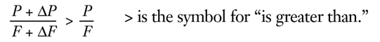
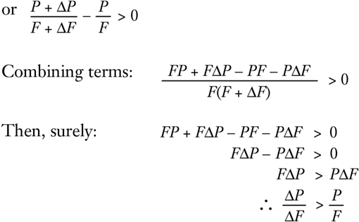
Thus, the MPP is greater than the old APP. Since it is greater, this means that there exists a positive number k such that:

Now there is an algebraic rule according to which, if:

then
Therefore,
Since k is positive,
Therefore,
In short, the MPP is also greater than the new APP.
In other words, if APP is increasing, then the marginal physical product is greater than the average physical product in this region. This proves the first law above. Now, if we go back in our proof and substitute “less than” signs for “greater than” signs and carry out similar steps, we arrive at the opposite conclusion: where APP is decreasing, the marginal physical product is lower than the average physical product. This proves the second of our three laws about the relation between the marginal and the average physical product. But if MPP is greater than APP when the latter is rising, and is lower than APP when the latter is falling, then it follows that when APP is at its maximum, MPP must be neither lower nor higher than, but equal to, APP. And this proves the third law. We see that these characteristics of our table apply to all possible cases of production.
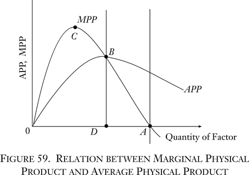
The diagram in Figure 59 depicts a typical set of MPP and APP schedules. It shows the various relationships between APP and MPP. Both curves begin from zero and are identical very close to their origin. The APP curve rises until it reaches a peak at B, then declines. The MPP curve rises faster, so that it is higher than APP, reaches its peak earlier at C, then declines until it intersects with APP at B. From then on, the MPP curve declines faster than APP, until finally it crosses the horizontal axis and becomes negative at some point A. No firm will operate beyond the 0A area.
Now let us explore further the area of increasing APP, between 0 and D. Let us take another hypothetical tabulation (Table 14), which will be simpler for our purpose.
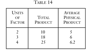
This is a segment of the increasing section of the average physical product schedule, with the peak being reached at four units and 6.2 APP. The question is: What is the likelihood that this region will be settled upon by a firm as the right input-output combination? Let us take the top line of the chart. Two units of the variable factor, plus a bundle of what we may call U units of all the other factors, yield 10 units of the product. On the other hand, at the maximum APP for the factor, four units of it, plus U units of other factors, yield 25 units of the product. We have seen above that it is a fundamental truth in nature that the same quantitative causes produce the same quantitative effects. Therefore, if we halve the quantities of all of the factors in the third line, we shall get half the product. In other words, two units of the factor combined with U/2—with half of the various units of each of the other factors—will yield 12.5 units of the product.
Consider this situation. From the top line we see that two units of the variable factor, plus U units of given factors, yield 10 units of the product. But, extrapolating from the bottom line, we see that two units of the variable factor, plus U/2 units of given factors, yield 12.5 units of the product. It is obvious that, as in the case of going beyond 0A, any firm that allocated factors so as to be in the 0D region would be making a most unwise decision. Obviously, no one would want to spend more in effort or money on factors (the “other” factors) and obtain less total output or, for that matter, the same total output. It is evident that if the producer remains in the 0D region, he is in an area of negative marginal physical productivity of the other factors. He would be in a situation where he would obtain a greater total product by throwing away some of the other factors. In the same way, after 0A, he would be in a position to gain greater total output if he threw away some of the present variable factor. A region of increasing APP for one factor, then, signifies a region of negative MPP for other factors, and vice versa. A producer, then, will never wish to allocate his factor in the 0D region or in the region beyond A.
Neither will the producer set the factor so that its MPP is at the points B or A. Indeed, the variable factor will be set so that it has zero marginal productivity (at A) only if it is a free good. There is however, no such thing as a free good; there is only a condition of human welfare not subject to action, and therefore not an element in productivity schedules. Conversely, the APP is at B, its maximum for the variable factor, only when the other factors are free goods and therefore have zero marginal productivity at this point. Only if all the other factors were free and could be left out of account could the producer simply concentrate on maximizing the productivity of one factor alone. However, there can be no production with only one factor, as we saw in chapter 1.
The conclusion, therefore, is inescapable. A factor will always be employed in a production process in such a way that it is in a region of declining APP and declining but positive MPP— between points D and A on the chart. In every production process, therefore, every factor will be employed in a region of diminishing MPP and diminishing APP so that additional units of the factor employed in the process will lower the MPP, and decreased units will raise it.
- 7It might be asked why we now employ mathematics after our strictures against the mathematical method in economics. The reason is that, in this particular problem, we are dealing with a purely technological question. We are not dealing with human decisions here, but with the necessary technological conditions of the world as given to human factors. In this external world, given quantities of cause yield given quantities of effect, and it is this sphere, very limited in the overall praxeological picture, that, like the natural sciences in general, is peculiarly susceptible to mathematical methods. The relationship between average and marginal is an obviously algebraic, rather than an ends-means, relation. Cf. the algebraic proof in Stigler, Theory of Price, pp. 44 ff.
C. Marginal Value Product
C. Marginal Value ProductAs we have seen, the MVP for any factor is its MPP multiplied by the selling price of its product. We have just concluded that every factor will be employed in its region of diminishing marginal physical product in each process of production. What will be the shape of the marginal value product schedule? As the supply of a factor increases, and other factors remain the same, it follows that the total physical output of the product is greater. A greater stock, given the consumers’ demand curve, will lead to a lowering of the market price. The price of the product will then fall as the MPP diminishes and rise as the latter increases. It follows that the MVP curve of the factor will always be falling, and falling at a more rapid rate than the MPP curve. For each specific production process, any factor will be employed in the region of diminishing MVP.8 This correlates with the previous conclusion, based on the law of utility, that the factor in general, among various production processes, will be employed in such a way that its MVP is diminishing. Therefore, its general MVP (between various uses and within each use) is diminishing, and its various particular MVPs are diminishing (within each use). Its DMVP is, therefore, diminishing as well.
The price of a unit of any factor will, as we have seen, be established in the market as equal to its discounted marginal value product. This will be the DMVP as determined by the general schedule including all the various uses to which it can be put. Now the producers will employ the factor in such a way that its DMVP will be equalized among all the uses. If the DMVP in one use is greater than in another, then employers in the former line of production will be in a position to bid more for the factor and will use more of it until (according to the principle of diminishing MVP) the DMVP of the expanding use diminishes to the point at which it equals the increasing DMVP in the contracting use. The price of the factor will be set as equal to the general DMVP, which in the ERE will be uniform throughout all the particular uses.
Thus, by looking at a factor in all of its interrelations, we have been able to explain the pricing of its unit service without previously assuming the existence of the price itself. To focus the analysis on the situation as it looks from the vantage point of the firm is to succumb to such an error, for the individual firm obviously finds a certain factor price given on the market. The price of a factor unit will be established by the market as equal to its marginal value product, discounted by the rate of interest for the length of time until the product is produced, provided that this valuation of the share of the factor is isolable. It is isolable if the factor is nonspecific or is a single residual specific factor in a process. The MVP in question is determined by the general MVP schedule covering the various uses of the factor and the supply of the factor available in the economy. The general MVP schedule of a factor diminishes as the supply of the factor increases; it is made up of particular MVP schedules for the various uses of the factor, which in turn are compounded of diminishing Marginal Physical Product schedules and declining product prices. Therefore, if the supply of the factor increases, the MVP schedule in the economy remaining the same, the MVP and hence the price of the factor will drop; and as the supply of the factor dwindles, ceteris paribus, the price of the factor will rise.
To the individual firm, the price of a factor established on the market is the signal of its discounted marginal value product elsewhere. This is the opportunity cost of the firm’s using the product, since it equals the value product that is forgone through failure to use the factor unit elsewhere. In the ERE, where all factor prices equal discounted marginal value products, it follows that factor prices and (opportunity) “costs” will be equal.
Critics of the marginal productivity analysis have contended that in the “modern complex world” all factors co-operate in producing a product, and therefore it is impossible to establish any sort of imputation of part of the product to various co-operating factors. Hence, they assert, “distribution” of product to factors is separable from production and takes place arbitrarily according to bargaining theory. To be sure, no one denies that many factors do co-operate in producing goods. But the fact that most factors (and all labor factors) are nonspecific, and that there is very rarely more than one purely specific factor in a production process, enables the market to isolate value productivity and to tend to pay each factor in accordance with this marginal product. On the free market, therefore, the price of each factor is not determined by “arbitrary” bargaining, but tends to be set strictly in accordance with its discounted marginal value product. The importance of this market process becomes greater as the economy becomes more specialized and complex and the adjustments more delicate. The more uses develop for a factor, and the more types of factors arise, the more important is this market “imputation” process as compared to simple bargaining. For it is this process that causes the effective allocation of factors and the flow of production in accordance with the most urgent demands of the consumers (including the nonmonetary desires of the producers themselves). In the free-market process, therefore, there is no separation between production and “distribution.” There is no heap somewhere on which “products” are arbitrarily thrown and from which someone does or can arbitrarily “distribute” them among various people. On the contrary, individuals produce goods and sell them to consumers for money, which they in turn spend on consumption or on investment in order to increase future consumption. There is no separate “distribution”; there is only production and its corollary, exchange.
It should always be understood, even where it is not explicitly stated in the text for reasons of exposition, that the MVP schedules used to set prices are discounted MVP schedules, discounting the final MVP by the length of time remaining until the final consumers’ product is produced. It is the DMVPs that are equalized throughout the various uses of the factor. The importance of this fact is that it explains the market allocation of nonspecific factors among various productive stages of the same or of different goods. Thus, if the DMVP of a factor is six gold ounces, and if the factor is employed on a process practically instantaneous with consumption, its MVP will be six. Suppose that the pure rate of interest is 5 percent. If the factor is at work on a process that will mature in final consumption five years from now, a DMVP of six signifies an MVP of 7.5; if it is at work on a 10-year process, a DMVP of six signifies an MVP of 10; etc. The more remote the time of operation is from the time when the final product is completed, the greater must be the difference allowed for the annual interest income earned by the capitalists who advance present goods and thereby make possible the entire length of the production process. The amount of the discount from the MVP is greater here because the higher stage is more remote than the others from final consumption. Therefore, in order for investment to take place in the higher stages, their MVP has to be far higher than the MVP in the shorter processes.9
3. The Source of Factor Incomes
3. The Source of Factor IncomesOur analysis permits us now to resolve that time-honored controversy in economics: Which is the source of wages—capital or consumption? Or, as we should rephrase it, which is the source of original-factor incomes (for labor and land factors)? It is clear that the ultimate goal of the investment of capital is future consumption. In that sense, consumption is the necessary requisite without which there would be no capital. Furthermore, for each particular good, consumption dictates, through market demands, the prices of the various products and the shifting of (nonspecific) factors from one process to another. However, consumption by itself provides nothing. Savings and investment are needed in order to permit any consumption at all, since very little consumption could be obtained with no production processes or capital structure at all—perhaps only the direct picking of berries.10
In so far as labor or land factors produce and sell consumers’ goods immediately, no capital is required for their payment. They are paid directly by consumption. This was true for Crusoe’s berry-picking. It is also true in a highly capitalistic economy for labor (and land) in the final stages of the production process. In these final stages, which include pure labor incomes earned in the sale of personal services (of doctors, artists, lawyers, etc.) to consumers, the factors earn MVP directly without being discounted in advance. All the other labor and land factors participating in the production process are paid by saved capital in advance of the produced and consumed product.
We must conclude that in the dispute between the classical theory that wages are paid out of capital and the theory of Henry George, J.B. Clark, and others that wages are paid out of the annual product consumed, the former theory is correct in the overwhelming majority of cases, and that this majority becomes more preponderant the greater the stock of capital in the society.11
4. Land and Capital Goods
4. Land and Capital GoodsThe price of the unit service of every factor, then, is equal to its discounted marginal value product. This is true of all factors, whether they be “original” (land and labor) or “produced” (capital goods). However, as we have seen, there is no net income to the owners of capital goods, since their prices contain the prices of the various factors that co-operate in their production. Essentially, then, net income accrues only to owners of land and labor factors and to capitalists for their “time” services. It is still true, however, that the pricing principle—equality to discounted MVP—applies whatever the factor, whether capital good or any other.
Let us revert to the diagram in Figure 41. This time, let us assume for simplicity that we are dealing with one unit of one consumers’ good, which sells for 100 ounces, and that one unit of each particular factor enters into its production. Thus, on Rank 1, 80 refers to one unit of a capital good. Let us consider the first rank first. Capitalistsl purchase one capital good for 80 ounces and (we assume) one labor factor for eight ounces and one land factor for seven ounces. The joint MVP for the three factors is 100. Yet their total price is 95 ounces. The remainder is the discount accruing to the capitalists because of the time element. The sum of the discounted MVPs, then, is 95 ounces, and this is precisely what the owners of three factors received in total. The discounted MVP of the labor factor’s service was eight, the DMVP of the land’s service was seven, the DMVP of the capital good’s service was 80. Thus, each factor obtains its DMVP as its received price. But what happens in the case of the capital good? It has been sold for 80, but it has had to be produced, and this production cost money to pay the income of the various factors. The price of the capital good, then, is reduced to, say, another land factor, paid eight ounces; another labor factor paid 8 ounces, and a capital-goods factor paid 60 ounces. The prices, and therefore the incomes, of all these factors are discounted again to account for the time, and this discount is earned by Capitalists2. The sum of these factor incomes is 76, and once again each factor service earns its DMVP.
Each capital-goods factor must be produced and must continue to be produced in the ERE. Since this is so, we see that the capital-goods factor, though obtaining its DMVP, does not earn it net, for its owner, in turn, must pay money to the factors that produce it. Ultimately, only land, labor, and time factors earn net incomes.
This type of analysis has been severely criticized on the following grounds:
This “Austrian” method of tracing everything back to land and labor (and time!) may be an interesting historical exercise, and we may grant that, if we trace back production and investment far enough, we shall ultimately reach the world of primitive men, who began to produce capital with their bare hands. But of what relevance is this for the modern, complex world around us, a world in which a huge amount of capital already exists and can be worked with? In the modern world there is no production without the aid of capital, and therefore the whole Austrian capital analysis is valueless for the modern economy.
There is no question about the fact that we are not interested in historical analysis, but rather in an economic analysis of the complex economy. In particular, acting man has no interest in the historical origin of his resources; he is acting in the present on behalf of a goal to be achieved in the future.12 Praxeological analysis recognizes this and deals with the individual acting at present to satisfy ends of varying degrees of futurity (from instantaneous to remote).
It is true, too, that the presentation by the master of capital and production theory, Böhm-Bawerk, sowed confusion by giving an historical interpretation to the structure of production. This is particularly true of his concept of the “average period of production,” which attempted to establish an average length of production processes operating at present, but stretching back to the beginning of time. In one of the weakest parts of his theory, Böhm-Bawerk conceded that “The boy who cuts a stick with his knife is, strictly speaking, only continuing the work of the miner who, centuries ago, thrust the first spade into the ground to sink the shaft from which the ore was brought to make the blade.”13 He then tried to salvage the relevance of the production structure by averaging periods of production and maintaining that the effect in the present product of the early centuries’ work is so small (being so remote) as to be negligible.
Mises has succeeded, however, in refining the Austrian production theory so as to eliminate reliance on an almost infinitely high production structure and on the mythical concept of an “average period of production.”
As Mises states:
Acting man does not look at his condition with the eyes of an historian. He is not concerned with how the present situation originated. His only concern is to make the best use of the means available today for the best possible removal of future uneasiness. ... He has at his disposal a definite quantity of material factors of production. He does not ask whether these factors are nature-given or the product of production processes accomplished in the past. It does not matter for him how great a quantity of nature-given, i.e., original material factors of production and labor, was expended in their production and how much time these processes of production have absorbed. He values the available means exclusively from the aspect of the services they can render him in his endeavors to make future conditions more satisfactory. The period of production and the duration of serviceableness are for him categories in planning future action, not concepts of academic retrospection. ... They play a role in so far as the actor has to choose between periods of production of different length. ...
[Böhm-Bawerk] ... was not fully aware of the fact that the period of production is a praxeological category and that the role it plays in action consists entirely in the choices acting man makes between periods of production of different length. The length of time expended in the past for the production of capital goods available today does not count at all.14
But if the past is not taken into account, how can we use the production-structure analysis? How can it apply to an ERE if the structure would have to go back almost endlessly in time? If we base our approach on the present, must we not follow the Knightians in scrapping the production-structure analysis?
A particular point of contention is the dividing line between land and capital goods. The Knightians, in scoffing at the idea of tracing periods of production back through the centuries, scrap the land concept altogether and include land as simply a part of capital goods. This change, of course, completely alters production theory. The Knightians point correctly, for example, to the fact that present-day land has many varieties and amounts of past labor “mixed” with it: canals have been dug, forests cleared, basic improvements have been made in the soil, etc. They assert that practically nothing is pure “land” anymore and therefore that the concept has become an empty one.
As Mises has shown, however, we can revise Böhm-Bawerk’s theory and still retain the vital distinction between land and capital goods. We do not have to throw out, as do the Knightians, the land baby with the average-period-of-production bathwater. We can, instead, reformulate the concept of “land.” Up to this point we have simply assumed land to be the original, nature-given factors. Now we must modify this, in keeping with our focus on the present and the future rather than the past. Whether or not a piece of land is “originally” pure land is in fact economically immaterial, so long as whatever alterations have been made are permanent—or rather, so long as these alterations do not have to be reproduced or replaced.15 Land that has been irrigated by canals or altered through the chopping down of forests has become a present, permanent given. Because it is a present given, not worn out in the process of production, and not needing to be replaced, it becomes a land factor under our definition. In the ERE, this factor will continue to give forth its natural powers unstinted and without further investment; it is therefore land in our analysis. Once this occurs, and the permanent are separated from the nonpermanent alterations, we see that the structure of production no longer stretches back infinitely in time, but comes to a close within a relatively brief span of time.16 The capital goods are those which are continually wearing out in the process of production and which labor and land factors must work to replace. When we consider physical wearing out and replacement, then, it becomes evident that it would not take many years for the whole capital-goods structure to collapse, if no work were done on maintenance and replacement, and this is true even in the modern, highly capitalist economy. Of course, the higher the degree of “capitalist” development and the more stages in production, the longer will it take for all the capital goods to wear out.16
The “permanence” with which we are dealing refers, of course, to the physical permanence of the goods, and not to the permanence of their value. The latter depends on the shifting desires of consumers and could never be called permanent. Thus, there might be a land factor uniquely and permanently suitable as a vineyard. It is land and remains so, therefore, indefinitely. If, at some time, the consumers should completely lose their taste for wine, and the land becomes valueless and no longer used, it is still a permanent factor, and therefore is land, although now submarginal. It should be noted that the “permanence” is relevant to present considerations of human action. A piece of land might give forth a permanent marginal (physical) product, without necessity of maintenance, and suddenly a volcano might erupt or a hurricane strike in the area, and the permanence could be destroyed. Such conceivable natural events, however, are not ex ante relevant to human action, and therefore from the point of view of action this land is rightly considered as “permanent,” until the natural changes occur.18 ,19
The concept of “land” as used throughout this book, then, is entirely different from the popular concept of land. Let us, in this section, distinguish between the two by calling the former economic land and the latter geographic land. The economic concept includes all nature-given sources of value: what is usually known as natural resources, land, water, and air in so far as they are not free goods. On the other hand, a large part of the value of what is generally considered “land”—i.e., that part that has to be maintained with the use of labor—is really a capital good.
That agricultural land is an example of the latter may surprise the reader who is likely to think of it as permanently productive. This is completely wrong; the marginal physical productivity of (geographic) land varies greatly in accordance with the amount of labor that is devoted to maintaining or improving the soil, as against such use or nonuse of the soil as leads to erosion and a lower MPP. The basic soil (and here we are referring to the soil that would remain now if maintenance were suspended, not to the soil as it was in the dim past before cultivation) is the land element, while the final product—which is popularly known as agricultural land—is usually a capital good containing this land element.
And Van Sickle and Rogge say about the soil:
Land, as the top 12 to 18 inches from which grains, vegetables, grasses, and trees draw almost their entire nourishment, is highly destructible. To p soil can be washed or blown away (eroded), or its organic and mineral content can be dissolved and drawn down out of reach of plant life (leached) in a relatively few years, unless great care is exercised in its use. It can also be rebuilt by careful husbandry. Hence it can be said of all soils ... that their maintenance requires saving.20
The indestructibility of land is much more clearly exemplified in what is commonly called “urban land.” For land in urban areas (and this includes suburban land, land for factories, etc.) clearly evinces one of its most fundamentally indestructible features: its physical space—its part of the surface of the earth. For the surface area of the earth is, except in rare cases, eternally fixed, as is the geographic position of each piece of geographic land on the surface. This eternally fixed, permanent, positional aspect of geographic land is called the site aspect of the land, or as Mises aptly puts it, “the land as standing room.” Since it is permanent and nonreproducible, it very clearly comes under the category of economic land. The permanence, once again, refers to its physical spatial aspect; its site values, of course, are always subject to change.21 Midtown Manhattan is on the same site—the same geographical location—now as it was in the 1600’s, although the monetary values accruing to it have changed.
Suppose that a piece of currently unused land can be used for various agricultural purposes or for urban purposes. In that case, a choice will be made according to its alternative values as nonreplaceable economic land: between its discounted MVP as a result of the fertility of its basic soil and its discounted MVP as an urban site. And if a decision must be made whether land now used in agriculture and being maintained for that purpose should remain in agriculture or be used as a site for building, the principles of choice are the same. The marginal value return to the agricultural or urban land is broken down by the owner of the land—the “landlord”—into the interest return on the capital maintenance and improvement and the discounted marginal value return to the basic economic land.
“Basic land” (or “ground land”) in this treatise refers to the soil without maintenance, in the case of agriculture, or the pure site without depreciating superstructure, in the case of urban land. The basic land, therefore, whether it be soil or site, earns for its owner an ultimate unit price, or rent, equaling its DMVP. Working on this basic land, labor and investment create a finished capital good. This capital good, like all capital goods, also earns unit rents equal to its DMVP. However, this earning is broken down (and relevantly so in the current market, not as an historical exercise) into basic land rent and interest return on the capital invested (as well, of course, as returns to labor that works on the basic land, i.e., labor’s wage or “rent-price,” equaling its DMVP). This capital-good land we have variously termed “geographic land,” “land in the popular sense,” “final land,” “finished land.” When we speak simply of “land,” on the other hand, we shall always be referring to the true economic land—the currently nature-given factor.
- 12This was realized by Carl Menger. See F.A. Hayek, “Carl Menger” in Henry W. Spiegel, ed., The Development of Economic Thought (New York: John Wiley, 1952), pp. 530 ff.
- 13Böhm-Bawerk, Positive Theory of Capital, p. 88.
- 14Mises, Human Action, pp. 477, 485f. Also see Menger, Principles of Economics, pp. 166–67.
- 15“Nonreplaceable” as a criterion for land, in contrast to capital goods, is not equivalent to “permanent.” “Permanent” is a subdivision of “non-replaceable.” It is clear that permanent improvements do not have to be replaced. However, depletable natural resources, such as coal, ores, etc., are not permanent, but are also nonreplaceable. The key question is whether a resource has to be produced, in which case it earns only gross rents. If it does not or cannot, it earns net rents as well. Resources that are being depleted obviously cannot be replaced and are therefore land, not capital goods. See the section on depletable resources below.
- 16a16bWe may use “permanent” and “nonpermanent” in this section, because resources that are being depleted obviously cannot be included in any evenly rotating equilibrium. For more on depletable resources, see below. With depletable resources left aside, “permanent” becomes identical with “nonreproducible.”
- 18Neither is there any relation between the present issue of permanence or nonpermanence and the cosmological question of the permanence of matter and energy. See Mises, Human Action, p. 634.
- 19Stigler charges that the various distinctions between land and capital goods based on permanence or origin, such as are discussed herein, are physical rather than economic. These strictures miss the point. No one denies that these homogeneous factors can change greatly in value over time. But whether or not a given factor is original or improved, or permanent or needing to be maintained, is a physical question, and one that is very relevant to economic analysis. Certainly, the Knightian argument that all land is capital goods, because no land is original, is also an argument in the physical realm. Stigler, Production and Distribution Theories, p. 274.
- 20John V. Van Sickle and Benjamin A. Rogge, Introduction to Economics (New York: D. Van Nostrand, 1954), p. 141.
- 21But while the position is permanent, even the land itself was necessarily altered by man to prepare it for urban use. See chapter 2 above.
5. Capitalization and Rent
5. Capitalization and RentThe subject of “rent” is one of the most confused in the entire economic literature. We must, therefore, reiterate the meaning of rent as set forth above. We are using “rent” to mean the unit price of the services of any good. It is important to banish any preconceptions that apply the concept of rent to land only. Perhaps the best guide is to keep in mind the well-known practice of “renting out.” Rent, then, is the same as hire: it is the sale and purchase of the unit services of any good.22 It therefore applies as well to prices of labor services (called “wages”) as it does to land or to any other factor. The rent concept applies to all goods, whether durable or nondurable. In the case of a completely nondurable good, which vanishes fully when first used, its “unit” of service is simply identical in size with the “whole” good itself. In regard to a durable good, of course, the rent concept is more interesting, since the price of the unit service is distinguishable from the price of the “good as a whole.” So far, in this work, we have been assuming that no durable producers’ goods are ever bought outright, that only their unit services are exchanged on the market. Therefore, our entire discussion of pricing has dealt with rental pricing. It is obvious that the rents are the fundamental prices. The marginal utility analysis has taught us that men value goods in units and not as wholes; the unit price (or “rent”) is, then, the fundamental price on the market.
In chapter 4 we analyzed rental pricing and the price of the “good as a whole” for durable consumers’ goods. The principle is precisely the same for producers’ goods. The rental value of the unit service is the basic one, the one ultimately determined on the market by individual utility scales. The price of the “whole good,” also known as the capital value of the good, is equal to the sum of the expected future rents discounted by what we then vaguely called a time-preference factor and which we now know is the rate of interest. The capital value, or price of the good as a whole, then, is completely dependent on the rental prices of the good, its physical durability, and the rate of interest.23 Obviously, the concept of “capital value” of a good has meaning only when that good is durable and does not vanish instantly upon use. If it did vanish, then there would only be pure rent, without separate valuations for the good as a whole. When we use the term “good as a whole,” we are not referring to the aggregate supply of the whole good in the economy. We are referring, e.g., not to the total supply of housing of a certain type, but to one house, which can be rented out over a period of time. We are dealing with units of “whole goods,” and these units, being durable, are necessarily larger than their constituent unit services, which can be rented out over a period of time.
The principle of the determination of “capital values,” i.e., prices of “whole goods,” is known as capitalization, or the capitalizing of rents. This principle applies to all goods, not simply capital goods, and we must not be misled by similarity of terminology. Thus, capitalization applies to durable consumers’ goods, such as houses, TV sets, etc. It also applies to all factors of production, including basic land. The rental price, or rent, of a factor of production is equal, as we have seen, to its discounted marginal value product. The capital value of a “whole factor” will be equal to the sum of its future rents, or the sum of its DMVPs.24 This capital value will be the price for which the “whole good” will exchange on the market. It is at this capital value that a unit of a “whole good” such as a house, a piano, a machine, an acre of land, etc., will sell on the market. There is clearly no sense to capitalization if there is no market, or price, for the “whole good.” The capital value is the appraised value set by the market on the basis of rents, durability, and the interest rate.
The process of capitalization can encompass many units of a “whole good,” as well as one unit. Let us consider the example of chapter 4, section 7, and generalize from it to apply, not only to houses, but to all durable producers’ goods. The good is a 10-year good; expected future rents are 10 gold ounces per year (determined by consumer utilities for consumers’ goods, or by MVPs for producers’ goods). The rate of interest is 10 percent per annum. The present capital value of this good is 59.4 gold ounces. But this “whole good” is itself a unit of a larger supply; one of many houses, machines, plants, etc. At any rate, since all units of a good have equal value, the capital value of two such houses, or two such machines, etc., added together equals precisely twice the amount of one, or 118.8 ounces. Since we are adding rents or DMVPs in money terms, we may keep adding them to determine capital values of larger aggregates of durable goods. As a matter of fact, in adding capital values, we do not need to confine ourselves to the same good. All we need do is to add the capital values in whatever bundle of durable goods we are interested in appraising. Thus, suppose a firm, Jones Construction Company, wishes to sell all its assets on the market. These assets, necessarily durable, consist of the following:
- 3 machines. Each machine has a capital value (based on the sum of the DMVPs) of 10 ounces. Therefore, total capital value is 30 ounces.
- 1 building, with a capital value of 40 ounces.
- 4 acres of land. Each acre has a capital value of 10 ounces. Total is40 ounces.
- Total capital value of these assets: 110 ounces.
But we must always remember, in adding capital values, that these are relevant only in so far as they are expressed in market price or potential market price. Many writers have fallen into the trap of assuming that they can, in a similar way, add up the entire capital value of the nation or world and arrive at a meaningful figure. Estimates of National Capital or World Capital, however, are completely meaningless. The world, or country, cannot sell all its capital on the market. Therefore, such statistical exercises are pointless. They are without possible reference to the very goal of capitalization: correct estimation of potential market price.
As we have indicated, capitalization applies to all factors of production, or rather, to all factors where there are markets for the whole goods that embody them. We may call these markets capital markets. They are the markets for exchange of ownership, total or partial, of durable producers’ goods. Let us take the case of capital goods. The rent of a capital good is equal to its DMVP. The capitalized value of the capital good is the sum of the future DMVPs, or the discounted sum of the future MVPs. This is the present value of the good, and this is what the good will sell for on the capital market.
The process of capitalization, because it permeates all sectors of the economy, and because it is flexible enough to include different types of assets—such as the total capital assets of a firm—is a very important one in the economy. Prices of shares of the ownership of this capital will be set at their proportionate fraction of the total capital value of the assets. In this way, given the MVPs, durability, and the rate of interest, all the prices on the capital market are determined, and these will be the prices in the ERE. This is the way in which the prices of individual capital goods (machines, buildings, etc.) will be set on the market, and this is the way in which these values will be summed up to set the price of a bundle of capital assets, similar and dissimilar. Share prices on the stock market will be set according to the proportion that they bear to the capitalized value of the firm’s total assets.
We have stated that all factors that can be bought and sold as “whole goods” on the market are capitalized. This includes capital goods, ground land, and durable consumers’ goods. It is clear that capital goods and durable consumers’ goods can be and are capitalized. But what of ground land? How can this be capitalized?
We have seen in detail above that the ultimate earnings of factors go to the owners of labor and of ground land and, as interest, to capitalists. If land can be capitalized, does this not mean that land and capital goods are “really the same thing” after all? The answer to the latter question is No.25 It is still emphatically true that the earnings of basic land factors are ultimate and irreducible, as are labor earnings, while capital goods have to be constantly produced and reproduced, and therefore their earnings are always reducible to the earnings of ground land, labor, and time.
Basic land can be capitalized for one simple reason: it can be bought and sold “as a whole” on the market. (This cannot be done for labor, except under a system of slavery, which, of course, cannot occur on the purely free market.) Since this can be and is being done, the problem arises how the prices in these exchanges are determined. These prices are the capital values of ground land.
A major characteristic of land as compared to capital goods is that its series of future rents is generally infinite, since, whether as basic soil or site, it is physically indestructible. In the ERE, the series of future rents will, of course, always be the same. The very fact that any land is ever bought and sold, by the way, is a demonstration of the universality of time preference. If there were no time preference for the present, then an infinite series of future rents could never be capitalized. A piece of land would have to have an infinite present price and therefore could never be sold. The fact that lands do have prices is an indication that there is always a time preference and that future rents are discounted to reduce to a present value.
As in the case of any other good, the capital value of land is equal to the sum of its discounted future rents. For example, it can be demonstrated mathematically that if we have a constant rent expected to be earned in perpetuity, the capital value of the asset will equal the annual rent divided by the rate of interest.26 Now it is obvious that on such land, the investor annually obtains the market rate of interest. If, in other words, annual rents will be 50, and the rate of interest is 5 percent, the asset will sell for 50/.05, or 1,000. The investor who purchases the asset for 1,000 ounces will earn 50 ounces a year from it, or 5 percent, the market rate of interest.
Ground land, then, is “capitalized” just as are capital goods, shares in capital-owning firms, and durable consumers’ goods. All these owners will tend to receive the same rate of interest return, and all will receive the same rate of return in the ERE. In short, all owned assets will be capitalized. In the ERE, of course, the capital values of all assets will remain constant; they will also be equal to the discounted sum of the MVPs of their unit rents.
Above, we saw that a key distinction between land and capital goods is that the owners of the former sell future goods for present money, whereas the owners of the latter advance present money, buy future goods, and later sell their product when it is less distantly future. This is still true. But then we must ask the question: How does the landowner come to own this land? The answer is (excepting his or his ancestors’ finding unused land and putting it to use) that he must have bought it from someone else. If he did so, then, in the ERE, he must have bought it at its capitalized value. If he buys the piece of land at a price of 1,000 ounces, and receives 50 ounces per annum in rent, then he earns interest, and only interest. He sells future goods (land service) in the production process, but he too first bought the whole land with money. Therefore, he too is a “capitalist-investor” earning interest.
“Pure rent,” i.e., rent that is not simply a return on previous investment and is therefore not capitalized, seems, therefore, to be earned only by those who have found unused land themselves (or inherited it from the finders). But even they do not earn pure rent. Suppose that a man finds land, unowned and worth zero, and then fences it, etc., until it is now able to yield a perpetual rental of 50 ounces per annum. Could we not say that he earns pure rent, since he did not buy the land, capitalized, from someone else? But this would overlook one of the most important features of economic life: implicit earnings. Even if this man did not buy the land, the land is now worth a certain capital value, the one it could obtain on the market. This capital value is, say, 1,000. Therefore, the man could sell the land for 1,000 at any time. His forgone opportunity cost of owning the land and renting out its services is sale of the land for 1,000 ounces. It is true that he earns 50 ounces per year, but this is only at the sacrifice of not selling the whole land for 1,000 ounces. His land, therefore, is really as much capitalized as land that has been bought on the market.
We must therefore conclude that no one receives pure rent except laborers in the form of wages, that the only incomes in the productive ERE economy are wages (the term for the prices and incomes of labor factors) and interest. But there is still a crucial distinction between land and capital goods. For we see that a fundamental, irreducible element is the capital value of land. The capital value of capital goods still reduces to wages and the capital value of land. In a changing economy, there is another source of income: increases in the capital value of ground land. T y p ical was the man who found unused land and then sold its services. Originally, the capital value of the land was zero; it was worthless. Now the land has become valuable because it earns rents. As a result, the capital value has risen to 1,000 ounces. His income, or gain, consisted of the rise of 1,000 ounces in capital value. This, of course, cannot take place in the ERE. In the ERE, all capital values must remain constant; here, we see that a source of monetary gain is a rise in the capital value of land, a rise resulting from increases in expected rental yields of land.27 If the economy becomes an ERE after this particular change from zero to 1,000, then this income was a “one-shot” affair, rather than a continuing and recurring item. The capital value of the land rose from zero to 1,000, and the owner can reap this income at any time. However, after this has been reaped once, it is never reaped again. If he sells the land for 1,000, the next buyer receives no gain from the increase in capital value; he receives only market interest. Only interest and wages accrue continuously. As long as the ERE continues, there will be no further gains or losses in capital value.28
- 22This concept of rent is based on the original contribution of Frank A. Fetter. Cf. Fetter, Economic Principles, pp. 143–70. Fetter’s conception has, unfortunately, had little influence on economic thought. It is not only in accord with common usage; it provides a unifying principle, enabling a coherent explanation of the price determination of unit services and of the whole goods that embody them. Without the rental-price concept, it is difficult to distinguish between the pricing of unit services and of whole goods.
Fetter used the rental concept to apply only to the services of durable goods, but it is clear that it can be extended to cover cases of nondurable goods where the unit service is the whole good. - 23See chapter 4 above. On capitalization, see Fetter, Economic Principles, pp. 262–84, 308–13; and Böhm-Bawerk, Positive Theory of Capital, pp. 339–57.
- 24It is often more convenient to define rent as equal to the MVP, rather than the DMVP. In that case, the capital value of the whole factor is equal to the discounted sum of its future rents.
- 25Fetter’s main error in capital theory was his belief that capitalization meant the scrapping of any distinction between capital goods and land.
- 26Cf. Boulding, Economic Analysis, pp. 711–12.
- 27In the long run, increases in the capital value of capital goods are unimportant, since they resolve into increases in wages and increases in the capital value of ground land.
- 28The problem of gains from changes in capital values will be treated further below.
6. The Depletion of Natural Resources
6. The Depletion of Natural ResourcesOne category has been purposely omitted so far from the discussion of land factors. At first, we defined land as the original, nature-given factor. Then we said that land which had been improved by human hands but which is now permanently given must also be considered as land. Land, then, became the catallactically permanent, nonreproducible resource, while capital goods are those that are nonpermanent and therefore must be produced again in order to be replaced. But there is one type of resource that is nonreplaceable but also nonpermanent: the natural resource that is being depleted, such as a copper or a diamond mine. Here the factor is definitely original and nature-given; it cannot be produced by man. On the other hand, it is not permanent, but subject to depletion because any use of it leaves an absolutely smaller amount for use in the future. It is original, but nonpermanent. Shall it be classed as land or as a capital good?
The crucial test of our classificatory procedure is to ask: Must labor and land factors work in order to reproduce the good? In the case of permanent factors this is not necessary, since they do not wear out. But in this case, we must answer in the negative also, for these goods, though nonpermanent, cannot be reproduced by man despite their depletion. Therefore, the natural resource comes as a special division under the “land” category.29
Table 15, adapted from one by Professor Hayek, reveals our classification of various resources as either land or capital goods.30

Hayek criticizes the criterion of reproducibility for classifying a capital good. He declares: “The point that is relevant ... is not that certain existing resources can be replaced by others which are in some technological sense similar to them, but that they have to be replaced by something, whether similar or not, if the income stream is not to decline.”31
But this is confusing value with physical considerations. We are attempting to classify physical goods here, not to discuss their possible values, which will fluctuate continually. The point is that the resources subject to depletion cannot be replaced, much as the owner would like to do so. They therefore earn a net rent. Hayek also raises the question whether a stream is “land” if a new stream can be created by collecting rain water. Here again, Hayek misconceives the issue as one of maintaining a “constant income stream” instead of classifying a physical concrete good. The stream is land because it does not need to be physically replaced. It is obvious that Hayek’s criticism is valid against Kaldor’s definition. Kaldor defined capital as a reproducible resource which it is economically profitable to produce. In that case, obsolete machines would no longer be capital goods. (Would they be “land”?) The definition should be: physically reproducible resources. Hayek’s criticism that then the possibility of growing artificial fruit, etc., would make all land “capital” again misconceives the problem, which is one of the physical need and possibility of reproducing the agent. Since the basic land—not its fruit—needs no reproduction, it is excluded from the capital-good category.
The fact that the natural resources cannot be reproduced means that they earn a net rent and that their rent is not absorbed by land and labor factors that go into their production. Of course, from the net rents they earn the usual interest rate of the society for their owners, interest earnings being related to their capital value. Increases in capital values of natural resources go ultimately to the resource-owner himself and are not absorbed in gains by other land and labor factors.
There is no problem in capitalizing a resource that is subject to depletion, since, as we have seen, capitalization can take place for either a finite or an infinite series of future rental incomes.
There is, however, one striking problem that pervades any analysis of the resource subject to depletion and that distinguishes it from all other types of goods. This is the fact that there can be no use for such a resource in an evenly rotating economy. For the basis of the ERE is that all economic quantities continue indefinitely in an endless round. But this cannot happen in the case of a resource that is subject to depletion, for whenever it is used, the total stock of that good in the economy decreases. The situation at the next moment, then, cannot be the same as before. This is but one example of the insuperable difficulties encountered whenever the ERE is used, not as an auxiliary construction in analysis, but as some sort of ideal that the free economy must be forced to emulate.
There can be a reserve demand for a depletable resource, just as there is speculative reserve demand for any other stock of goods on the market. This speculation is not simple wickedness, however; it has a definite function, namely, that of allocating the scarce depletable resource to those uses at those times when consumer demand for them will be greatest. The speculator, waiting to use the resources until a future date, benefits consumers by shifting their use to a time when they will be more in demand than at present. As in the case of ground land, the permanent resource belongs to the first finder and first user, and often some of these initial capital gains are absorbed by interest on the capital originally invested in the business of resource-finding. The absorption can take place only in so far as the finding of new resources is a regular, continuing business. But this business, which by definition could not exist in the ERE, can never be completely regularized.
Minerals such as coal and oil are clearly prime examples of depletable resources. What about such natural resources as forests? A forest, although growing by natural processes, can be “produced” by man if measures are taken to maintain and grow more trees, etc. Therefore, forests would have to be classified as capital goods rather than depletable resources.
One of the frequent attacks on the behavior of the free market is based on the Georgist bugbear of natural resources held off the market for speculative purposes. We have dealt with this alleged problem above. Another, and diametrically opposite, attack is the common one that the free market wastes resources, especially depletable resources. Future generations are allegedly robbed by the greed of the present. Such reasoning would lead to the paradoxical conclusion that none of the resource be consumed at all. For whenever, at any time, a man consumes a depletable resource (here we use “consumes” in a broader sense to include “uses up” in production), he is leaving less of a stock for himself or his descendants to draw upon. It is a fact of life that whenever any amount of a depletable resource is used up, less is left for the future, and therefore any such consumption could just as well be called “robbery of the future,” if one chooses to define robbery in such unusual terms.32 Once we grant any amount of use to the depletable resource, we have to discard the robbery-of-the-future argument and accept the individual preferences of the market. There is then no more reason to assume that the market will use the resources too fast than to assume the opposite. The market will tend to use resources at precisely the rate that the consumers desire.33
Having developed, in Volume I, our basic analysis of the economics of the isolated individual, barter, and indirect exchange, we shall now proceed, in Volume II, to develop the analysis further by dealing with “dynamic” problems of a changing economy, particular types of factors, money and its value, and monopoly and competition, and discussing, in necessarily more summary fashion, the consequences of violent intervention in the free market.
- 29Cf. Fred R. Fairchild, Edgar S. Furniss, and Norman S. Buck, Elementary Economics (New York: Macmillan & Co., 1926), II, 147.
- 30Hayek, Pure Theory of Capital, p. 58 n.
- 31Ibid., p. 58 n.
- 32Unusual terms because robbery has been distinctively defined as seizure of someone else’s property without his consent, not the use of one’s own property.
- 33As Stigler says in discussing the charge of “wasted” resources on the market, “It is an interesting problem to define ‘wasteful’ sensibly without making the word synonymous with ‘unprofitable.’” Stigler, Theory of Price, p. 332 n. For a discussion of natural resources and a critique of the doctrines of “conservation,” see Anthony Scott, Natural Resources: The Economics of Conservation (Toronto: University of Toronto Press, 1955).
Appendix A: Marginal Physical and Marginal Value Product
Appendix A: Marginal Physical and Marginal Value ProductFor purposes of simplification, we have described marginal value product (MVP) as equal to marginal physical product (MPP) times price. Since we have seen that a factor must be used in the region of declining MPP, and since an increased supply of a factor leads to a fall in price, the conclusion of the analysis was that every factor works in an area where increased supply leads to a decline in MVP, and hence in DMVP. The assumption made in the first sentence, however, is not strictly correct.
Let us, then, find out what is the multiple of MPP that will yield an MVP. MVP is equal to an increase in revenue acquired from the addition of a unit, or lost from the loss of a unit, of a factor. MVP will then equal the difference in revenue from one position to another, i.e., the change in position resulting from an increase or decrease of a unit of a factor. Then, MVP equals R2 – R1, where R is the gross revenue from the sale of a product, and a higher subscript signifies that more of a factor has been used in production. The MPP of this increase in a factor is P2 – P1, where P is the quantity of product produced, a higher subscript again meaning that more of a factor has been used.
Revenue is acquired by sale of the product; therefore, for any given point on the demand curve, total revenue equals the quantity produced and sold, multiplied by the price of the product.
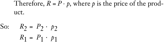
Now, since the factors are economic goods, any increase in the use of a factor, other factors remaining constant, must increase the quantity produced. It would obviously be pointless for an entrepreneur to employ more factors which would not increase the product. Therefore, P2 > P1.
On the other hand, the price of the product falls as the supply increases, so that:
p2 < p1
Now, we are trying to find out what multiplied by MPP yields MVP. This unknown will be equal to:
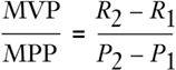
This may be called the marginal revenue, which is the change in revenue divided by the change in output.
It is obvious that this figure. which we may call MR, will not equal either p2 or p1, or any average of the two. Simple multiplication of the denominator by either of the p‘s or both will reveal that this does not amount to the numerator. What is the relation between MR and price?
A price is the average revenue, i.e., it equals the total revenue divided by the quantity produced and sold. In short,

But above, in the discussion of marginal and average product, we saw the mathematical relationship between “average” and “marginal,” and this holds for revenue as well as for productivity: namely, that in the range where the average is increasing, marginal is greater than average; in the range where average is decreasing, marginal is less than average. But we have established early in this book that the demand curve—i.e., the price, or average revenue curve—is always falling as the quantity increases. Therefore, the marginal revenue curve is falling also and is always below average revenue, or price. Let us, however, cement the proof by demonstrating that, for any two positions, p2 is greater than MR. Since p2 is smaller than p1, as price falls when supply increases, the proposition that MR is less than both prices will be proved.
First, we know that p2 < p1, which means that

Now, we may take point one as the starting point and then consider the change to point two, so that:
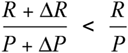
thus translating into the same symbols we used in the productivity proof above. Now this means that
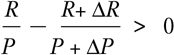
Combining the two fractions, and then multiplying across, we get
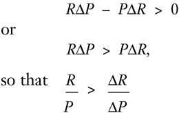
(We have here proved that MR is less than p1, the higher of the two prices.)
Now this means that there is some unknown, constant positive fraction l/k which, multiplied by the larger, will yield the smaller ratio (MR) in the last inequality. Thus,
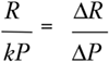
Now, by algebra,
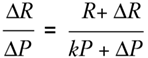
and since k is a positive number,
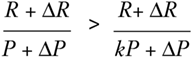
But this establishes that
i.e., that MR is less than p2. Q.E.D.
Hence, when we consider that, strictly, MR, and not price, should be multiplied by MPP to arrive at MVP, we find that our conclusion—that production always takes place in the zone of a falling MVP curve—is strengthened rather than weakened. MVP falls even more rapidly in relation to MPP than we had been supposing. Furthermore, our analysis is not greatly modified, because no new basic determinants—beyond MPP and prices set by the consumer demand curve—have been introduced in our corrective analysis. In view of all this, we may continue to treat MVP as equaling MPP times price as a legitimate, simplified approximation to the actual result.34
- 34A curious notion has arisen that considering MR, instead of price, as the multiplier somehow vitiates the optimum satisfaction of consumer desires on the market. There is no genuine warrant for such an assumption.
Appendix B: Professor Rolph and the Discounted Marginal Productivity Theory
Appendix B: Professor Rolph and the Discounted Marginal Productivity TheoryOf current schools of economic thought, the most fashionable have been the Econometric, the Keynesian, the Institutionalist, and the Neo-Classic. “Neo-Classic” refers to the pattern set by the major economists of the late nineteenth century. The dominant neoclassical strain at present is to be found in the system of Professor Frank Knight, of which the most characteristic feature is an attack on the whole concept of time preference. Denying time preference, and basing interest return solely on an alleged “productivity” of capital, the Knightians attack the doctrine of the discounted MVP and instead advocate a pure MVP theory. The clearest exposition of this approach is to be found in an article by a follower of Knight’s, Professor Earl Rolph.35
Rolph defines “product” as any immediate results of “present valuable activities.” These include work on goods that will be consumed only in the future. Thus,
workmen and equipment beginning the construction of a building may have only a few stakes in the ground to show for their work the first day, but this and not the completed structure is their immediate product. Thus, the doctrine that a factor receives the value of its marginal product refers to this immediate product. The simultaneity of production and product does not require any simplifying assumptions. It is a direct appeal to the obvious. Every activity has its immediate results.
Obviously, no one denies that people work on goods and move capital a little further along. But is the immediate result of this a product in any meaningful sense? It should be clear that the product is the end product—the good sold to the consumer. The whole purpose of the production system is to lead to final consumption. All the intermediate purchases are based on the expectation of final purchase by the consumer and would not take place otherwise. Every activity may have its immediate “results,” but they are not results that would command any monetary income from anyone if the owners of the factors themselves were joint owners of all they produced until the final consumption stage. In that case, it would be obvious that they do not get paid immediately; hence, their product is not immediate. The only reason that they are paid immediately (and even here there is not strict immediacy) on the market is that capitalists advance present goods in exchange for those future goods for which they expect a premium, or interest return. Thus, the owners of the factors are paid the discounted value of their marginal product.
The Knight-Rolph approach, in addition, is a retreat to a real-cost theory of value. It assumes that present efforts will somehow always bring present results. But when? In “present valuable activities.” But how do these activities become valuable? Only if their future product is sold, as expected, to consumers. Suppose, however, that people work for years on a certain good and are paid by capitalists, and then the final product is not bought by consumers. The capitalists absorb monetary losses. Where was the immediate payment according to marginal product? The payment was only an investment in future goods by capitalists.
Rolph then turns to another allegedly heinous error of the discount approach, namely, the “doctrine of nonco-ordination of factors.” This means that some factors, in their payment, receive the discounted value of their product and some do not. Rolph, however, is laboring under a misapprehension; there is no assumption of nonco-ordination in any sound discounting theory. As we have stated above, all factors—labor, land, and capital goods—receive their discounted marginal value product. The difference in regard to the owners of capital goods is that, in the ultimate analysis, they do not receive any independent payment, since capital goods are resolved into the factors that produced them, ultimately land and labor factors, and to interest for the time involved in the advance of payment by the capitalists.36 Rolph believes that nonco-ordination is involved because owners of land and labor factors “receive a discounted share,” and capital “receives an undiscounted share.” But this is a faulty way of stating the conclusion. Owners of land and labor factors receive a discounted share, but owners of capital (money capital) receive the discount.
The remainder of Rolph’s article is largely devoted to an attempt to prove that no time lag is involved in payments to owners of factors. Rolph assumes the existence of “production centers” within every firm, which, broken down into virtually instantaneous steps, produce and then implicitly receive payment instantaneously. This tortured and unreal construction misses the entire point. Even if there were atomized “production centers,” the point is that some person or persons will have to make advances of present money along the route, in whatever order, until the final product is sold to the consumers. Let Rolph picture a production system, atomized or integrated as the case may be, with no one making the advances of present goods (money capital) that he denies exist. And as the laborers and landowners work on the intermediate products for years without pay, until the finished product is ready for the consumer, let Rolph exhort them not to worry, since they have been implicitly paid simultaneously as they worked. For this is the logical implication of the Knight-Rolph position.37
- 35Earl Rolph, “The Discounted Marginal Productivity Doctrine” in W. Fellner and B.F. Haley, eds., Readings in Theory of Income Distribution (Philadelphia: Blakiston, 1946), pp. 278–93.
- 36Rolph ascribes this error to Knut Wicksell, but such a confusion is not attributable to Wicksell, who engages in a brilliant discussion of capital and the production structure and the role of time in production. Wicksell demonstrates correctly that labor and land are the only ultimate factors, and that therefore the marginal productivity of capital goods is reducible to the marginal productivity of labor and land factors, so that money capital earns the interest (or discount) differential.
Wicksell’s discussion of these and related issues is of basic importance. He recognized, for example, that capital goods are fully and basically coordinate with land and labor factors only from the point of view of the individual firm, but not when we consider the total market in all of its interrelations. Current economic theorizing is, to its detriment, even more preoccupied than writers of his day with the study of an isolated firm instead of the interrelated market. Wicksell, Lectures on Political Economy, I, 148–54, 185–95. - 37Rolph ends his article, consistently, with a dismissal of any time-preference influences on interest, which he explains in Knightian vein by the “cost” of producing new capital goods.